Chi-square (χ2) is used to test hypotheses about the distribution of observations into categories with no inherent ranking.
What Is a Chi-Square Statistic?
The Chi-square test (pronounced Kai) looks at the pattern of observations and will tell us if certain combinations of the categories occur more frequently than we would expect by chance, given the total number of times each category occurred.
It looks for an association between the variables. We cannot use a correlation coefficient to look for the patterns in this data because the categories often do not form a continuum.
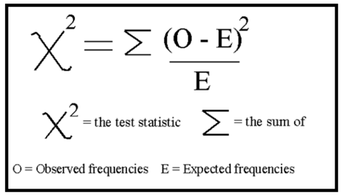
There are three main types of Chi-square tests, tests of goodness of fit, the test of independence, and the test for homogeneity. All three tests rely on the same formula to compute a test statistic.
These tests function by deciphering relationships between observed sets of data and theoretical or “expected” sets of data that align with the null hypothesis.
What is a Contingency Table?
Contingency tables (also known as two-way tables) are grids in which Chi-square data is organized and displayed. They provide a basic picture of the interrelation between two variables and can help find interactions between them.
In contingency tables, one variable and each of its categories are listed vertically, and the other variable and each of its categories are listed horizontally.
Additionally, including column and row totals, also known as “marginal frequencies,” will help facilitate the Chi-square testing process.
In order for the Chi-square test to be considered trustworthy, each cell of your expected contingency table must have a value of at least five.
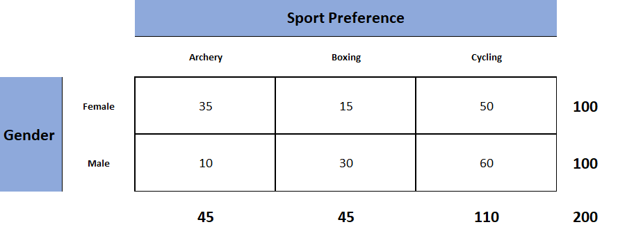
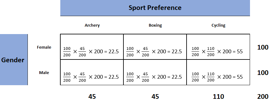
Each Chi-square test will have one contingency table representing observed counts (see Fig. 1) and one contingency table representing expected counts (see Fig. 2).

Figure 1. Observed table (which contains the observed counts).
To obtain the expected frequencies for any cell in any cross-tabulation in which the two variables are assumed independent, multiply the row and column totals for that cell and divide the product by the total number of cases in the table.

Figure 2. Expected table (what we expect the two-way table to look like if the two categorical variables are independent).
To decide if our calculated value for χ2 is significant, we also need to work out the degrees of freedom for our contingency table using the following formula: df= (rows – 1) x (columns – 1).
Formula Calculation

Calculate the chi-square statistic (χ2) by completing the following steps:
- Calculate the expected frequencies and the observed frequencies.
- For each observed number in the table, subtract the corresponding expected number (O — E).
- Square the difference (O —E)².
- Divide the squares obtained for each cell in the table by the expected number for that cell (O – E)² / E.
- Sum all the values for (O – E)² / E. This is the chi-square statistic.
- Calculate the degrees of freedom for the contingency table using the following formula; df= (rows – 1) x (columns – 1).
Once we have calculated the degrees of freedom (df) and the chi-squared value (χ2), we can use the χ2 table (often at the back of a statistics book) to check if our value for χ2 is higher than the critical value given in the table. If it is, then our result is significant at the level given.
Interpretation
The chi-square statistic tells you how much difference exists between the observed count in each table cell to the counts you would expect if there were no relationship at all in the population.
Small Chi-Square Statistic: If the chi-square statistic is small and the p-value is large (usually greater than 0.05), this often indicates that the observed frequencies in the sample are close to what would be expected under the null hypothesis.
The null hypothesis usually states no association between the variables being studied or that the observed distribution fits the expected distribution.
In theory, if the observed and expected values were equal (no difference), then the chi-square statistic would be zero — but this is unlikely to happen in real life.
Large Chi-Square Statistic: If the chi-square statistic is large and the p-value is small (usually less than 0.05), then the conclusion is often that the data does not fit the model well, i.e., the observed and expected values are significantly different. This often leads to the rejection of the null hypothesis.
How to Report
To report a chi-square output in an APA-style results section, always rely on the following template:
χ2 ( degrees of freedom, N = sample size ) = chi-square statistic value, p = p value .

In the case of the above example, the results would be written as follows:
A chi-square test of independence showed that there was a significant association between gender and post-graduation education plans, χ2 (4, N = 101) = 54.50, p < .001.
APA Style Rules
- Do not use a zero before a decimal when the statistic cannot be greater than 1 (proportion, correlation, level of statistical significance).
- Report exact p values to two or three decimals (e.g., p = .006, p = .03).
- However, report p values less than .001 as “ p < .001.”
- Put a space before and after a mathematical operator (e.g., minus, plus, greater than, less than, equals sign).
- Do not repeat statistics in both the text and a table or figure.
p -value Interpretation
You test whether a given χ2 is statistically significant by testing it against a table of chi-square distributions, according to the number of degrees of freedom for your sample, which is the number of categories minus 1. The chi-square assumes that you have at least 5 observations per category.
If you are using SPSS then you will have an expected p -value.
For a chi-square test, a p-value that is less than or equal to the .05 significance level indicates that the observed values are different to the expected values.
Thus, low p-values (p< .05) indicate a likely difference between the theoretical population and the collected sample. You can conclude that a relationship exists between the categorical variables.
Remember that p -values do not indicate the odds that the null hypothesis is true but rather provide the probability that one would obtain the sample distribution observed (or a more extreme distribution) if the null hypothesis was true.
A level of confidence necessary to accept the null hypothesis can never be reached. Therefore, conclusions must choose to either fail to reject the null or accept the alternative hypothesis, depending on the calculated p-value.
Using SPSS
The four steps below show you how to analyze your data using a chi-square goodness-of-fit test in SPSS (when you have hypothesized that you have equal expected proportions).
Step 1: Analyze > Nonparametric Tests > Legacy Dialogs > Chi-square… on the top menu as shown below:
Step 2: Move the variable indicating categories into the “Test Variable List:” box.
Step 3: If you want to test the hypothesis that all categories are equally likely, click “OK.”
Step 4: Specify the expected count for each category by first clicking the “Values” button under “Expected Values.”
Step 5: Then, in the box to the right of “Values,” enter the expected count for category one and click the “Add” button. Now enter the expected count for category two and click “Add.” Continue in this way until all expected counts have been entered.
Step 6: Then click “OK.”
The four steps below show you how to analyze your data using a chi-square test of independence in SPSS Statistics.
Step 1: Open the Crosstabs dialog (Analyze > Descriptive Statistics > Crosstabs).
Step 2: Select the variables you want to compare using the chi-square test. Click one variable in the left window and then click the arrow at the top to move the variable. Select the row variable and the column variable.
Step 3: Click Statistics (a new pop-up window will appear). Check Chi-square, then click Continue.
Step 4 : (Optional) Check the box for Display clustered bar charts.
Step 5: Click OK.
Goodness-of-Fit Test
The Chi-square goodness of fit test is used to compare a randomly collected sample containing a single, categorical variable to a larger population.
This test is most commonly used to compare a random sample to the population from which it was potentially collected.
The test begins with the creation of a null and alternative hypothesis. In this case, the hypotheses are as follows:
Null Hypothesis (Ho): The null hypothesis (Ho) is that the observed frequencies are the same (except for chance variation) as the expected frequencies. The collected data is consistent with the population distribution.
Alternative Hypothesis (Ha): The collected data is not consistent with the population distribution.
The next step is to create a contingency table that represents how the data would be distributed if the null hypothesis were exactly correct.
The sample’s overall deviation from this theoretical/expected data will allow us to draw a conclusion, with a more severe deviation resulting in smaller p-values.
Test for Independence
The Chi-square test for independence looks for an association between two categorical variables within the same population.
Unlike the goodness of fit test, the test for independence does not compare a single observed variable to a theoretical population but rather two variables within a sample set to one another.
The hypotheses for a Chi-square test of independence are as follows:
Null Hypothesis (Ho): There is no association between the two categorical variables in the population of interest.
Alternative Hypothesis (Ha): There is no association between the two categorical variables in the population of interest.
The next step is to create a contingency table of expected values that reflects how a data set that perfectly aligns the null hypothesis would appear.
The simplest way to do this is to calculate the marginal frequencies of each row and column; the expected frequency of each cell is equal to the marginal frequency of the row and column that corresponds to a given cell in the observed contingency table divided by the total sample size.
Test for Homogeneity
The Chi-square test for homogeneity is organized and executed exactly the same as the test for independence.
The main difference to remember between the two is that the test for independence looks for an association between two categorical variables within the same population, while the test for homogeneity determines if the distribution of a variable is the same in each of several populations (thus allocating population itself as the second categorical variable).
The hypotheses for a Chi-square test of independence are as follows:
Null Hypothesis (Ho): There is no difference in the distribution of a categorical variable for several populations or treatments.
Alternative Hypothesis (Ha): There is a difference in the distribution of a categorical variable for several populations or treatments.
The difference between these two tests can be a bit tricky to determine, especially in the practical applications of a Chi-square test. A reliable rule of thumb is to determine how the data was collected.
If the data consists of only one random sample with the observations classified according to two categorical variables, it is a test for independence. If the data consists of more than one independent random sample, it is a test for homogeneity.
FAQs
What is the chi-square test?
The Chi-square test is a non-parametric statistical test used to determine if there’s a significant association between two or more categorical variables in a sample.
It works by comparing the observed frequencies in each category of a cross-tabulation with the frequencies expected under the null hypothesis, which assumes there is no relationship between the variables.
This test is often used in fields like biology, marketing, sociology, and psychology for hypothesis testing.
What does chi-square tell you?
The Chi-square test informs whether there is a significant association between two categorical variables. Suppose the calculated Chi-square value is above the critical value from the Chi-square distribution.
In that case, it suggests a significant relationship between the variables, rejecting the null hypothesis of no association.
How to calculate chi-square?
To calculate the Chi-square statistic, follow these steps:
1. Create a contingency table of observed frequencies for each category.
2. Calculate expected frequencies for each category under the null hypothesis.
3. Compute the Chi-square statistic using the formula: Χ² = Σ [ (O_i – E_i)² / E_i ], where O_i is the observed frequency and E_i is the expected frequency.
4. Compare the calculated statistic with the critical value from the Chi-square distribution to draw a conclusion.

