Properties of normal distribution
The normal distribution is a continuous probability distribution that is symmetrical on both sides of the mean, so the right side of the center is a mirror image of the left side.
The area under the normal distribution curve represents the probability and the total area under the curve sums to one.
Most of the continuous data values in a normal distribution tend to cluster around the mean, and the further a value is from the mean, the less likely it is to occur. The tails are asymptotic, which means that they approach but never quite meet the horizon (i.e., the x-axis).
For a perfectly normal distribution, the mean, median, and mode will be the same value, visually represented by the peak of the curve.
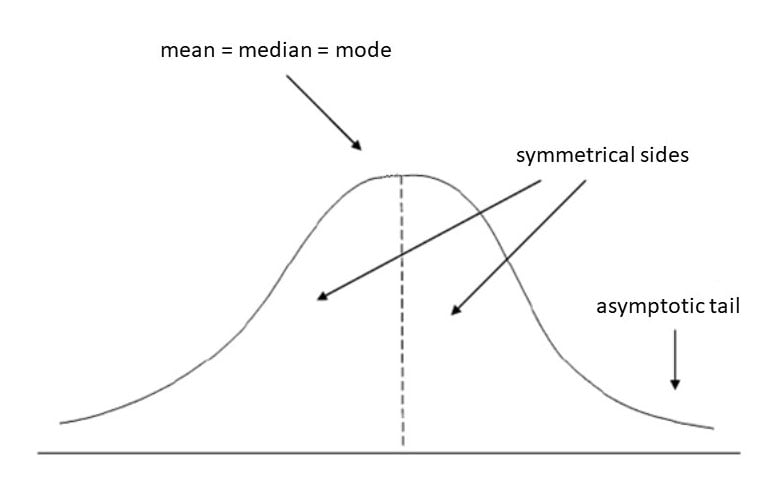
The normal distribution is often called the bell curve because the graph of its probability density looks like a bell. It is also known as called Gaussian distribution, after the German mathematician Carl Gauss who first described it.
Normal distribution Vs. Standard normal distribution?
A normal distribution is determined by two parameters the mean and the variance. A normal distribution with a mean of 0 and a standard deviation of 1 is called a standard normal distribution.
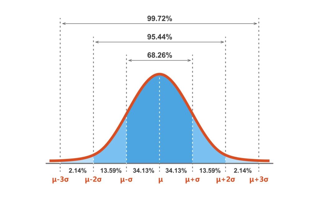
Figure 1. A standard normal distribution (SND).
This is the distribution that is used to construct tables of the normal distribution.
Why is the normal distribution important?
The bell-shaped curve is a common feature of nature and psychology
The normal distribution is the most important probability distribution in statistics because many continuous data in nature and psychology display this bell-shaped curve when compiled and graphed.
For example, if we randomly sampled 100 individuals, we would expect to see a normal distribution frequency curve for many continuous variables, such as IQ, height, weight, and blood pressure.
Parametric significance tests require a normal distribution of the sample’s data points
The most powerful (parametric) statistical tests psychologists use require data to be normally distributed. If the data does not resemble a bell curve, researchers may use a less powerful statistical test called non-parametric statistics.
Converting the raw scores of a normal distribution to z-scores
We can standardize a normal distribution’s values (raw scores) by converting them into z-scores.
This procedure allows researchers to determine the proportion of the values that fall within a specified number of standard deviations from the mean (i.e., calculate the empirical rule).
What is the empirical rule formula?
The empirical rule in statistics allows researchers to determine the proportion of values that fall within certain distances from the mean. The empirical rule is often referred to as the three-sigma rule or the 68-95-99.7 rule.
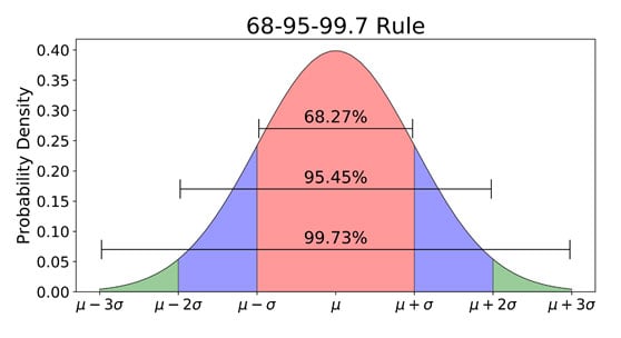
If the data values in a normal distribution are converted to standard score (z-score) in a standard normal distribution, the empirical rule describes the percentage of the data that fall within specific numbers of standard deviations (σ) from the mean (μ) for bell-shaped curves.
The empirical rule allows researchers to calculate the probability of randomly obtaining a score from a normal distribution.
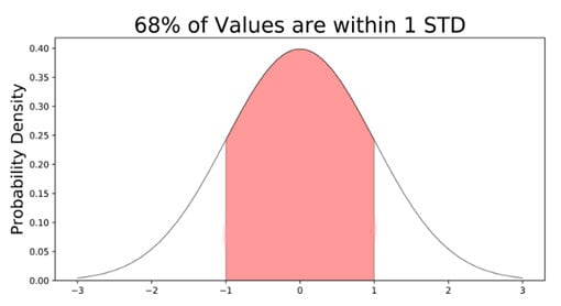
68% of data falls within the first standard deviation from the mean. This means there is a 68% probability of randomly selecting a score between -1 and +1 standard deviations from the mean.
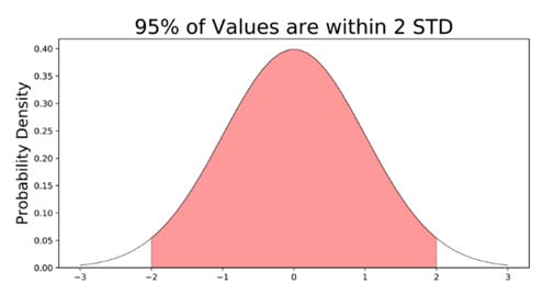
95% of the values fall within two standard deviations from the mean. This means there is a 95% probability of randomly selecting a score between -2 and +2 standard deviations from the mean.
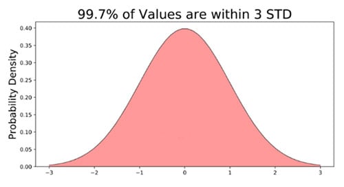
99.7% of data will fall within three standard deviations from the mean. This means there is a 99.7% probability of randomly selecting a score between -3 and +3 standard deviations from the mean.
How to check data
Statistical software (such as SPSS) can be used to check if your dataset is normally distributed by calculating the three measures of central tendency. If the mean, median, and mode are very similar values, there is a good chance that the data follows a bell-shaped distribution (SPSS command here).
It is also advisable to use a frequency graph too, so you can check the visual shape of your data (If your chart is a histogram, you can add a distribution curve using SPSS: From the menus, choose: Elements > Show Distribution Curve).
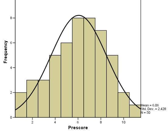
Normal distributions become more apparent (i.e., perfect) the finer the level of measurement and the larger the sample from a population.
You can also calculate coefficients which tell us about the size of the distribution tails in relation to the bump in the middle of the bell curve. For example, Kolmogorov Smirnov and Shapiro-Wilk tests can be calculated using SPSS.
These tests compare your data to a normal distribution and provide a p-value, which, if significant (p < .05), indicates your data is different from a normal distribution (thus, on this occasion, we do not want a significant result and need a p-value higher than 0.05).

Is a normal distribution kurtosis 0 or 3?
A normal distribution has a kurtosis of 3. However, sometimes people use “excess kurtosis,” which subtracts 3 from the kurtosis of the distribution to compare it to a normal distribution.
In that case, the excess kurtosis of a normal distribution would be be 3 − 3 = 0.
So, the normal distribution has kurtosis of 3, but its excess kurtosis is 0.

